FlyRank ML Internship · Lane 4 · Capstone
Which pages should an SEO editor review first?
Ranking 12,023 content items against a transparent baseline — and reporting the two claims that did not survive client-clustered resampling.
1Abstract
Content that ranks in search decays quietly — positions slip, clicks fall, and the
team notices late — and FlyRank, which publishes content into client sites and then
optimises it algorithmically, already surfaces decay candidates using hand-written threshold
rules; the open question is whether a learned ranking can order that candidate pool better than
the rule can, given an inventory far larger than any review budget. I built a ranked review
queue over 12,023 pseudonymised content items from 28 clients in the FlyRank ML Internship
dataset (~79M rows), using trailing-90-day search behaviour, with a separate warehouse window
used for genuine past → future validation. An eight-feature logistic regression — selected from 16 configurations under
nested cross-validation — was compared against a transparent hand-written rule on
client-grouped folds, and every comparison was bootstrapped twice: once resampling rows, and
once resampling clients. The learned scorer ranks measurably better than the rule (ROC AUC
0.631 vs 0.577; precision@50 0.90 vs 0.68 against a 0.599 base rate; ΔAUC +0.079 with a
client-clustered 95% interval of [0.021, 0.109]), but two further comparisons — against a
larger feature set, and against a one-line ctr == 0 heuristic — did not
survive client clustering and are reported here as retracted rather than dropped. The output is
decision support: a ranked queue with reason codes and a measured stopping point, past which the
queue is worse than no ordering at all.
2The problem: a to-do list 195× longer than the day
Where this comes from
FlyRank treats content as infrastructure: it researches, writes and publishes content directly into a client's website, then watches the search data and optimises — the whole cycle run by algorithms rather than by people working page by page. That model runs into one persistent difficulty. Content that gets found in search decays quietly. A page ranks, holds, and then slips: positions drift down, clicks fall away, and because nothing breaks visibly, most teams notice only after the traffic is gone. Across thousands of pages per client, the valuable decision is not is this page healthy? — it is which page should a human fix first?
FlyRank's product already answers a version of that question today, using hand-written threshold rules: a health score, quick-win tags, needs-attention flags. If-this-then-that, with the numbers chosen by hand. They work, and they run in production. But rules of that shape run out exactly where the signals get many, tangled, and shifting — and at the time of this study no trained model had replaced them. This capstone lives in that gap: it asks, on real production search data, whether a learned ranking can order the candidate pool better than the rule that produced it.
One consequence of that framing shaped the whole study, and it is worth stating plainly: product flags are the thing to beat, never a thing to learn from. A health score or a needs-attention tag encodes a decision someone has already made. Feeding it in as a feature would produce a model that predicts the company's own past choices and calls the result a finding. So the hand-written rule appears in this paper exclusively as the baseline, and every column that carries a trace of a prior editorial decision is in the exclusion table in §3.
What that looks like on a Monday morning
An editor sits down with time to properly review about fifty pages. The pipeline hands them a list of 9,759 — every page that clears a fixed threshold of at least 500 impressions, a visible position between 1 and 20, and a click-through rate under 0.5%. Each of those pages genuinely qualifies. The list is still useless, because it is roughly 195 times longer than the week.
That gap is the entire problem, and it is a ranking problem rather than a classification one. Nobody needs a correct yes/no verdict on all 12,023 items; they need a trustworthy ordering of the fifty that will actually be opened. So quality is measured at the top of the list — precision@50 — and that metric was named before any model existed, so it could not be shopped for afterwards.
A fixed rule cannot produce that ordering, because the same CTR number means opposite things depending on where the page sits. A 0.10% click-through rate is above the median for a page ranking on results page three, and less than half the norm for a page sitting at position four. In this dataset, at the same page-one position, comparison articles averaged ~0.14% CTR against ~0.35% for keyword articles — a 2.5× difference that position alone does not explain. Hand-writing thresholds for every (position tier × content type × volume bucket) cell means dozens of numbers, each drifting as the inventory changes. That is the shape of problem where a learned ranking earns its place — conditionally, and only if it beats the transparent rule on held-out clients.
The decision this supports. One content editor, one review cycle, a fixed budget of roughly fifty pages. The output is a ranked queue with a score, an archetype, and human-readable reason codes. A wrong call costs a wasted review slot — and, worse, the genuine under-performer that slot should have gone to. Nothing here is automated: the queue orders questions for a human, it does not answer them.
3Data
Everything below comes from the FlyRank ML Internship dataset, a pseudonymised release of roughly 79 million rows of production search and engagement data. Three surfaces of it are involved, and they are kept distinct on purpose.
| Surface | Tables | Window | Used for |
|---|---|---|---|
| Warehouse (queried in place via DuckDB) | fact_content_daily_performance (March 2026 partition, ~9.8M rows), dim_content, dim_clients |
features 2026-03-01 → 03-31, outcome April 2026 | Data contract, the leakage attacks, and the time-aware 2×2 |
| Starter slice (anonymised content-refresh extract) | one row per content item, trailing-90-day aggregates | trailing 90 days | The main 12,023-item study: baseline, model, folds, queue |
| Sealed | fact_content_daily_performance_sample (~11.7M rows) |
June 2026 | Never touched. Declared off-limits when the contract was written, and left alone |
Population, and the grain
One row is one pseudonymised content item for one client, described by its trailing 90-day search behaviour. Not a page-day, not a client — the editor's decision happens at the content-item level, so the model's rows live there too. The study population is visible pages only: at least 500 trailing-90-day impressions, at a real position between 1 and 20, GSC-measured. That is 12,023 content items across 28 clients, 40.1% of the starter release. One client alone accounts for 36.6% of those rows, a fact that shapes every uncertainty estimate later in this paper.
What was excluded, and why
Exclusions are the part of a data section that is worth reading, so here is the whole list.
| Column(s) | Category | Why excluded |
|---|---|---|
trend_direction, trend_pct, *_last_30d, *_prev_30d |
label components | The label is derived from these. A feature that builds the label is the label. |
any April column (ctr_apr, clk_apr, imp_apr) |
outcome window | Hasn't happened at decision time. Planted deliberately once as a leak test — AUC jumped to 0.993 — then removed. |
| any multi-month aggregate spanning the outcome window | window overlap | A "61-day CTR" looks like an innocent long-window feature and quietly contains the label window. |
ga4_*, sessions_*, scroll_events |
measurement gap | Zero-filled wherever GA4 was not connected. Those zeros mean "not measured", not "no engagement" — using them would teach the model which clients had GA4. |
ai_chatgpt, ai_perplexity, ai_gemini, ai_claude, … |
sparse, out of lane | Too sparse to support a claim here, and AI-referral analysis is a different lane's question. |
client_has_gsc, access_profile, is_active, client metadata |
client identity | Static per-client attributes encode which client a row belongs to — the one thing a cross-client model must not learn. |
last_optimized_date, optimization_eligible_date |
decision trace | Encodes "someone already decided to act on this page". Predicting your own product's past decisions is circular. |
search_volume, competition, cpc, keyword_* |
no measured signal | Search volume's correlation with actual impressions is ~0.001 in this slice. The obvious prioritisation signal carries nothing. |
client_hash_id, content_hash_id, url_hash_id |
pseudonymous IDs | Grouping, joining and splitting only. An ID in the feature matrix is memorisation by construction. |
Public-safety. No client names, domains, URLs, or raw search queries appear anywhere in this work. Client and content identifiers are pseudonyms used only for grouping, joining and splitting — never as features, and never printed on this page. The ranked queue itself carries those pseudonyms, so it is deliberately excluded from version control; only aggregate tables and metrics files are published.
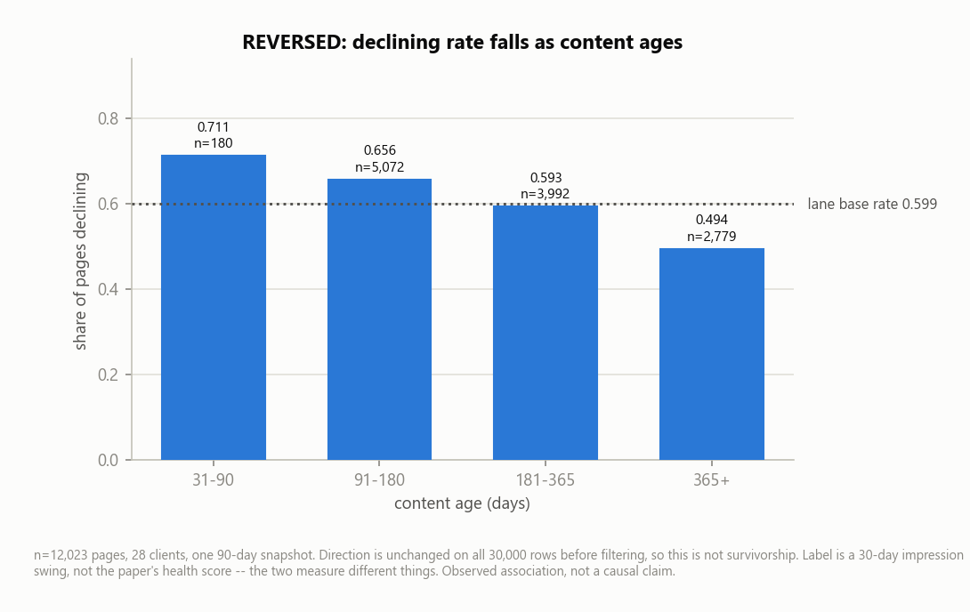
One structural feature of the inventory is worth showing before any modelling, because it is the pattern the queue is built to exploit and it is visible without a model at all.
4Methodology
Assumptions, stated so they can be attacked
- Review capacity is roughly fifty pages per cycle, so quality is measured at the top of the list, not averaged over 12,023 rows nobody will open.
- Position-conditioned comparison is mandatory. A 0.3% CTR is ordinary at position 40 and alarming at position 3; every CTR claim here is conditioned on position tier.
- Content items within a client share a site, a template and an audience, so they are not independent draws. Splits group by client, and uncertainty is clustered by client.
- The queue orders review attention. It has never been validated against the outcome of actually refreshing anything, so "worth looking at first" is the only verb it earns.
The label, and its honest name
The target is is_declining_label: the item's trailing 30-day impressions fell
versus the previous 30 days. Base rate 0.599 on this population. This is a
proxy, and its weakness is named in the limitations rather than buried: it
records a current-window movement, not a future outcome. The genuine
past → future design — features from one fortnight, outcome observed in the
next — exists separately, on the warehouse, and is reported in the results.
The label was also deliberately not defined by me. An early version of this project would have scored each page's CTR gap against its position peers and then called anything past a threshold an "underperformer". Training on that would teach a model to reproduce my own threshold and call the result a finding. The CTR gap is used as a transparent score in the baseline; the trained label comes from movement the world produced.
The baseline the model has to beat
A transparent hand-written rule: ctr_gap × log(impressions) × confidence —
how far below the position-tier median an item's CTR sits, weighted by volume leverage, because a
small CTR improvement on a high-traffic page yields more absolute clicks. No fitted weights, one
reason code, fully explainable to a non-technical editor. Its expected-CTR lookup table (position
tier × content type median) is refit on training rows only, so the rule never peeks at test data
either. If the model cannot beat this on the same rows and the same metric, the rule ships.
The model, chosen by search rather than by taste
Sixteen configurations — four feature sets crossed with four estimators — were compared under nested cross-validation. Two things came out of that search, and the second is more interesting than the first.
The end-to-end ROC AUC spread across all sixteen configurations was only 0.067, and the inner folds selected four distinct configurations across five outer folds. In other words the choice of model is not stable, which is itself a result: on this problem the feature set matters more than the estimator, and neither matters very much. That is the argument for shipping the smallest thing that works.
The scorer I recommend — called shipped throughout this paper as shorthand for
"the one this study selects", not "running in production", which nothing here is — is a
logistic regression on eight features: six numeric
— ctr, log_clicks_90d, days_with_sessions,
log_impressions_90d, content_age_days, ctr_gap — and
two categorical, position_tier and content_type. The Week-5 model used
eleven features, two of which (avg_position, days_since_last_update)
were later measured at 0.502 and 0.506 single-feature AUC. Those are coin flips, and they are
gone.
Validation, in three layers
- Client-grouped 5-fold. Whole clients are held out, so the model is always scored on clients it has never seen. The same pipeline was also run on random folds, and the gap between the two schemes measures memorisation directly.
- Client-clustered bootstrap (2,000 resamples). Every comparison gets both a row-resampled interval and a client-resampled one. Where they disagree, the client interval wins and the claim is retracted.
- Time-aware 2×2 on the warehouse: new clients × later period, so the cost of unseen clients and the cost of elapsed time are separated instead of confounded.
Leakage checks that were actually run
- A planted label-derived feature drove AUC to 0.993 — proof the harness can see leakage when it is there. Then it was removed.
- A planted overlapping-window feature (a 61-day CTR spanning the outcome window) got the same treatment.
- Single-feature AUC on every survivor: the strongest is
ctrat 0.598, the weakestavg_positionat 0.502. Nothing is remotely in the range of the planted leak. This replaced a Pearson correlation scan, which ordered the features differently and would have missed a threshold-shaped leak entirely. - Permutation importance on held-out rows replaced impurity importance, which had over-rated
scroll_rate— the same methodological correction I had asked of someone else's chart, applied to my own. - Adversarial validation AUC = 0.961. Clients are almost perfectly separable from one another. This is the number that makes a random row split indefensible on this data.
- Categorical proxy screen — and the one result I kept anyway. Each candidate
categorical was scored on how well it alone predicts which client a row belongs to.
content_typescores 0.913, and it is one of the two categorical features in the shipped model. That is high: it means content type is close to a partial stand-in for client identity in this inventory, because different clients publish different mixes of content. I kept it, because it is a genuine attribute of the page rather than an identifier, and dropping every feature correlated with client would leave almost nothing. The honest position is that this is a disclosed trade-off, not a clean result — and it is part of why the headline number is a client-clustered interval rather than a point estimate.
5Results
(a) Model versus baseline, same rows, same folds
Every ranker below was scored out-of-fold on client-grouped folds, against a base rate of 0.599. Lift is precision@K divided by the base rate: a lift of 1.00 means "no better than reading the lane in any order at all".
| Ranker | ROC AUC | PR AUC | p@10 | p@50 | p@100 | lift@50 |
|---|---|---|---|---|---|---|
| parsimonious logreg (8 feat) — shipped | 0.631 | 0.715 | 0.90 | 0.90 | 0.88 | 1.50 |
| ensemble (LR + RF rank-average) | 0.627 | 0.709 | 0.90 | 0.86 | 0.91 | 1.44 |
| logistic regression (Week 5, 11 feat) | 0.625 | 0.703 | 0.60 | 0.88 | 0.86 | 1.47 |
| random forest | 0.618 | 0.702 | 1.00 | 0.94 | 0.86 | 1.57 |
| baseline rule (Week 4, transparent) | 0.577 | 0.646 | 0.60 | 0.68 | 0.67 | 1.14 |
ctr == 0 one-liner | 0.478 | 0.611 | 0.70 | 0.76 | 0.75 | 1.27 |
Green marks the best value in each column — and it is not on the row I recommend. The random forest wins precision@10, precision@50 and lift@50 outright. I am recommending the model that loses the metric I named in advance, so that decision has to be argued rather than highlighted, and §5(c) is where it is argued: the two are not distinguishable once uncertainty is clustered by client (ΔROC AUC −0.009, interval [−0.032, +0.006]), and under time shift the forest pays roughly double — 0.154 ROC AUC for elapsed time against the logistic regression's 0.075. A 0.04 precision@50 lead that a bootstrap cannot distinguish is not worth twice the degradation in the only test resembling deployment. If you disagree with that trade, the forest is the defensible alternative and this table gives you the numbers to make the case.
Separately, the ctr == 0 one-liner is included because it is the cheapest
thing that could possibly work. It scores a respectable 0.76 at K=50 while ranking worse than
chance across the full list (ROC AUC 0.478). That combination is exactly why precision@K on its
own is not sufficient evidence — a good top-50 can sit on top of a broken ordering.
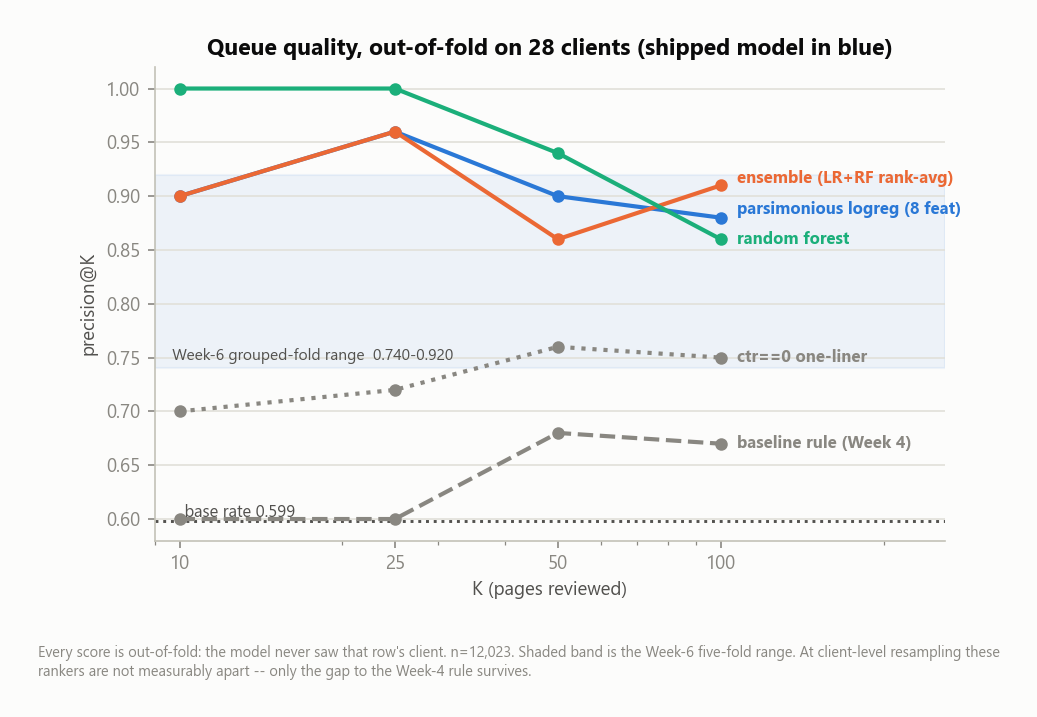
ctr == 0 one-liner, both of which track close to the 0.599 base rate line.(b) What the honest split cost
The same pipeline, the same rows, the same estimators, five folds each — the only thing that changes is how rows are assigned to folds.
| Model | p@50, random folds | p@50, client-grouped | optimism | grouped fold spread |
|---|---|---|---|---|
| random forest | 0.904 | 0.836 | +0.068 | 0.18 |
| logistic regression | 0.868 | 0.820 | +0.048 | 0.12 |
| baseline rule (Week 4) | 0.632 | 0.672 | −0.040 | 0.22 |
A reader handed only the random-split number would have inherited roughly seven points of optimism on the model I actually recommend. The control is the bottom row: the rule moved the other way. It has no client-specific structure to memorise, so it had nothing to lose — and that asymmetry is what localises the optimism to the models rather than to fold arithmetic.
(c) The result worth carrying: the simpler model travels better
Trained on one fortnight, tested on the next, with unseen clients and later period separated into their own cells. This is the only genuinely past → future evaluation in the study, and it changes which model you would deploy.
| Test cell | n | base rate | logreg ROC AUC | RF ROC AUC |
|---|---|---|---|---|
| same clients, same period | 14,462 | 0.374 | 0.676 | 0.729 |
| new clients, same period | 14,109 | 0.267 | 0.621 | 0.619 |
| same clients, later period | 50,928 | 0.642 | 0.601 | 0.575 |
| new clients, later period | 16,625 | 0.618 | 0.651 | 0.647 |
| Generalisation cost (ROC AUC paid) | logistic regression | random forest |
|---|---|---|
| cost of unseen clients | 0.054 | 0.110 |
| cost of elapsed time | 0.075 | 0.154 |
| cost of both at once | 0.025 | 0.083 |
The random forest wins the one cell that resembles the training distribution and loses every cell that resembles deployment, paying roughly double on each axis. The eight-feature logistic regression is not the more accurate model in-period; it is the one that survives leaving the period it was fitted in. On this evidence, that is the model to ship.
(d) What the model leans on, and where it is wrong
The importances below are permutation importances measured on the six held-out clients the model never saw, with one-hot blocks permuted together. That matters: an importance ranking taken on rows the model trained on answers a different question. They are measured on the Week-5 eleven-feature set, because that is the set the error analysis was run on.
Reading it in plain words: click-through rate is the model's main signal, content age
is second, and volume is third. Everything below the top three is close to noise —
positions 7 through 11 all sit under 0.004 AUC drop, which is the same scale as their own standard
deviations. This is also the check that corrects an earlier mistake of mine: Week 5 read
scroll_rate as the top feature using impurity importance, which is biased toward
high-cardinality continuous variables. On held-out rows it ranks fourth, and ctr
takes first. Two of eleven features moved by two or more ranks between the two methods.
| # | Feature | AUC drop when permuted | ± sd | In the shipped 8-feature set? |
|---|---|---|---|---|
| 1 | ctr | 0.0389 | 0.0035 | kept |
| 2 | content_age_days | 0.0291 | 0.0055 | kept |
| 3 | log_impressions_90d | 0.0256 | 0.0021 | kept |
| 4 | scroll_rate | 0.0145 | 0.0047 | dropped — GA4-derived, ~27% coverage |
| 5 | engagement_rate | 0.0119 | 0.0018 | dropped — GA4-derived, ~27% coverage |
| 6 | word_count_tier | 0.0048 | 0.0037 | dropped |
| 7 | avg_position | 0.0037 | 0.0013 | dropped — 0.502 alone, a coin flip |
| 8 | position_tier | 0.0035 | 0.0019 | kept |
| 9 | days_since_last_update | 0.0021 | 0.0017 | dropped — 0.506 alone |
| 10 | freshness_tier | 0.0006 | 0.0011 | dropped |
| 11 | content_type | 0.0003 | 0.0002 | kept |
The parsimonious set keeps the top three and discards most of the tail. The two
exceptions are deliberate and worth naming: scroll_rate and engagement_rate
rank fourth and fifth but are GA4-derived, and GA4 covers only about 27% of content items — keeping
them would trade a small measured gain for a large measurement-gap risk. content_type
is kept despite ranking last, because it carries the position-tier interaction the whole lane is
about; its client-identity trade-off is disclosed in §4.
Is ctr too important? The drop test
When one feature dominates, the honest question is whether it is a leak. Refitting without
ctr moves precision@50 from 0.820 to 0.700 and ROC AUC from 0.656 to
0.630 — the largest single-feature effect in the set, and it lands at the lower edge of the full
model's confidence interval. "Inside the interval" is a weak pass when the interval is 0.22 wide,
so I am not concluding ctr doesn't matter. It clearly does.
What the test does rule out is the thing it was built to rule out. A leaked feature has two
signatures and ctr has neither: it would rank near-perfectly alone (ctr
alone scores 0.598, and nothing in this feature set exceeds 0.60), and removing it
would collapse the model toward the base rate of 0.537 (without it the model still ranks at 0.700,
a lift of 1.30×). A strong legitimate feature and a leaked one both hurt when dropped; only the
leak scores near 1.0 on its own.
Where it is wrong — the 9 misses
On the six held-out clients the top-50 queue is 41 right, 9 wrong. The interesting part is what the wrong picks look like, compared against both reference classes — against the test-set average alone it is easy to describe a pattern that is really just "top of the queue".
| Feature | false positives (n=9) | true positives (n=41) | test set overall |
|---|---|---|---|
ctr | 0.07 | 0.06 | 0.35 |
scroll_rate | 18.65 | 17.45 | 9.45 |
content_age_days | 141.00 | 166.00 | 292.64 |
days_since_last_update | 65.33 | 60.12 | 54.90 |
avg_position | 5.31 | 4.66 | 10.83 |
impressions_90d | 2,373 | 1,829 | 9,012 |
engagement_rate | 0.00 | 0.60 | 3.93 |
Read the columns left to right: the wrong picks look almost exactly like the
right picks, and both look nothing like the test set. On CTR, scroll rate, age, position and
volume the two queue classes are nearly identical while differing sharply from the population. So the
model is good at separating "queue-worthy" from "ordinary" and comparatively poor at separating,
within the queue, which pages will actually decline. The single largest gap between the
misses and the hits is engagement_rate — 0.00 versus 0.60 — but that feature is
zero-inflated and is not in the shipped set, so it is a lead for the next iteration rather than a
fix available today. By content type, the nine misses were 7 keyword articles and 2 feedly articles;
no identifiers are involved.
The surprise worth keeping
The clearest directional finding in this study is one I did not expect and did not go looking for: decline rate falls monotonically as content ages — 0.711 in the 31–90 day tier down to 0.494 past a year, against a 0.599 base rate (chart in §3). The intuition that old pages are the decaying ones is backwards in this inventory. A plausible reading is survivorship in the ordinary sense — pages that have held their position for a year have already proven they can — and the effect direction is unchanged on all 30,000 rows before filtering, so it is not an artifact of the visible-pages filter. It remains an observed association on one inventory, with no causal claim attached.
6Limitations & honest framing
1. Two claims were retracted, and here they are
Every comparison was bootstrapped twice. Resampling rows assumes 12,023 independent draws; there are really 28 clients, one of which is 36.6% of the data. Resampling clients instead widens every interval, and two results that looked measurable stopped being measurable.
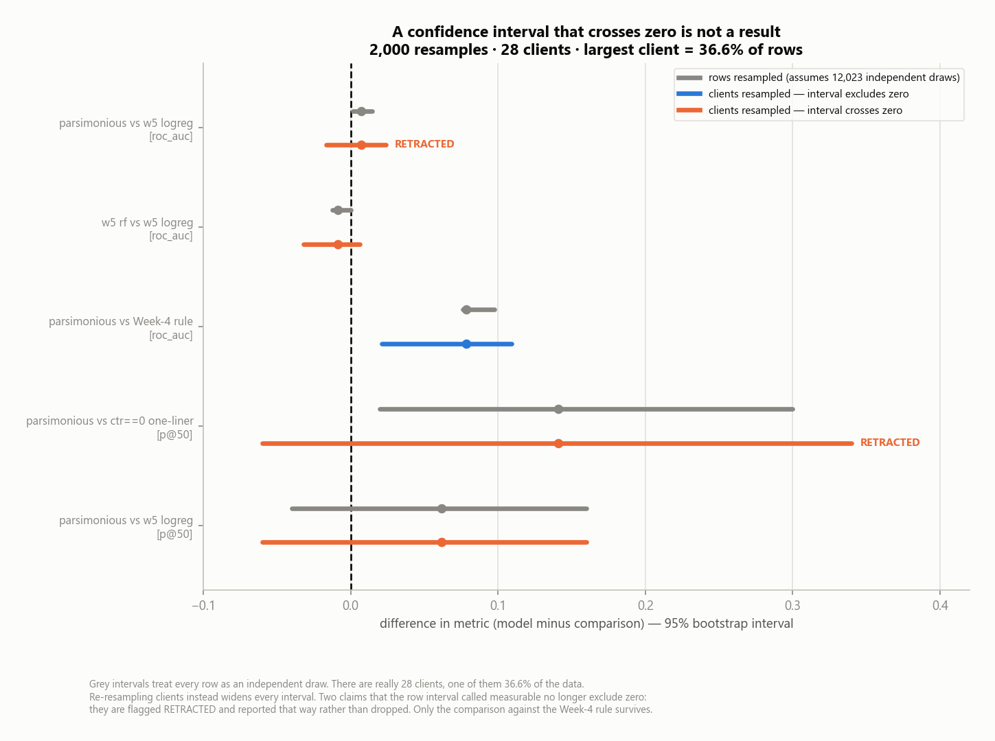
ctr == 0 one-liner at precision@50, do not — and are reported as retracted rather
than quietly removed.| Comparison | difference | rows resampled | clients resampled | verdict |
|---|---|---|---|---|
| shipped model vs Week-4 rule (ROC AUC) | +0.079 | [+0.076, +0.098] | [+0.021, +0.109] | holds |
| shipped model vs Week-5 11-feature model (ROC AUC) | +0.007 | [+0.001, +0.015] | [−0.017, +0.024] | RETRACTED — not distinguishable |
shipped model vs ctr == 0 one-liner (p@50) | +0.141 | [+0.020, +0.300] | [−0.060, +0.340] | RETRACTED — not distinguishable |
| shipped model vs Week-5 model (p@50) | +0.061 | [−0.040, +0.160] | [−0.060, +0.160] | never distinguishable |
| random forest vs logistic regression (ROC AUC) | −0.009 | [−0.013, +0.000] | [−0.032, +0.006] | never distinguishable |
Under client resampling the shipped scorer's absolute ROC AUC is [0.595, 0.673] and the Week-5 model's is [0.600, 0.659]. Those intervals overlap almost entirely. The case for the eight-feature model is parsimony and stability under time shift — not measured accuracy.
2. The label is a proxy, and a current-window one
is_declining_label records that trailing 30-day impressions fell against the prior
30 days. It is not "this page will decline", and it is emphatically not "refreshing this page will
help". In the warehouse fortnight-to-fortnight design, the base rate moved from
0.349 to 0.633 between two consecutive fortnights — a shift larger than
every model-versus-baseline gap in this entire study. Any deployment must measure its own base
rate before trusting a precision number.
3. Two shipped features drift by construction
days_since_update shows a population stability index of 8.49
between fortnights, and content_age_days 0.177, against a retrain trigger of 0.25.
These features encode "how long since a timestamp", so they drift as the calendar moves, whatever
the content does. They are in the shipped feature set. That is a named liability, not an
oversight, and it is the first thing a monitoring system here should watch.
4. Twenty-eight clients is a small n, and one is a third of it
The client-clustered intervals above are wide because they should be. With 28 clusters and one dominating, a single unusual client moves the estimate. Every headline in this paper is an interval, not a point.
5. No experiment exists anywhere in this work
Every number is observational and cross-sectional. Nothing here shows that rewriting a title raises click-through rate — that would need a controlled test that was never run. Nothing here observes a search engine's ranking function either; this data sees one inventory's outcomes, never the algorithm that produced them. The queue has never been validated against the result of actually refreshing anything, so "worth looking at first" is the strongest verb it earns.
6. The model is a ranker, not a decision — and it cannot see the page
The scorer sees eight numbers about a page. It has never seen the page. All eight
reason codes name something it structurally cannot check — that is why each one has a
written reviewer instruction attached rather than an action: stale_90plus means a
timestamp moved, not that anything changed; decay_zone_age means old, not stale;
thin_for_tier means short, not thin; ctr_gap_vs_peers means the click
rate is below the peer group's, not that the snippet actually mismatches the query;
striking_distance means position 11–20, not that the gap is realistically closable.
A concise definition page is not a thin page, and evergreen content is not dated content.
Competitive difficulty and query intent are not in the feature set at all. Every item is a
question for a human.
7. Not production
There is no API, no scheduler, no model registry and no automated action anywhere in this work. The deliverable is a ranked queue a person reads, plus the numeric rules for when to stop trusting it.
7Ranked recommendations
Ordered by how much evidence sits behind each one, strongest first, with the confidence stated rather than implied.
1. Review the top 50 each cycle — and know where the queue stops paying (measured)
Precision holds at 0.90 through K=50, 0.88 at K=100, 0.84 at K=400 and 0.79 at K=1,600. But cumulative precision hides the real story; marginal precision by decile shows it. Decile 1 runs at 0.809 (+0.211 over base rate) and decile 6 has already fallen below base rate. Past roughly rank 6,010, working down the queue is worse than reading the inventory in no particular order. Stop there.
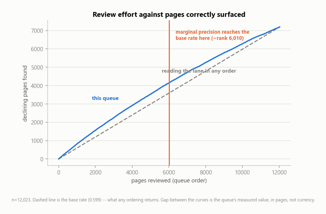
2. Ship the eight-feature logistic regression, not the forest (measured, with a stated overlap)
It beats the transparent rule by a margin that survives client clustering, and it degrades at roughly half the forest's rate under time shift. It is not measurably better than the larger Week-5 model — so the honest argument for it is parsimony and stability, not accuracy.
3. Keep the transparent rule running alongside it (measured)
The rule is the revert target, and the trigger is already a number rather than a feeling: if precision@50 falls to 0.672 or below, the rule is matching the model, and the rule is cheaper and explainable to anyone. Below 0.599 — the base rate — retire the queue entirely.
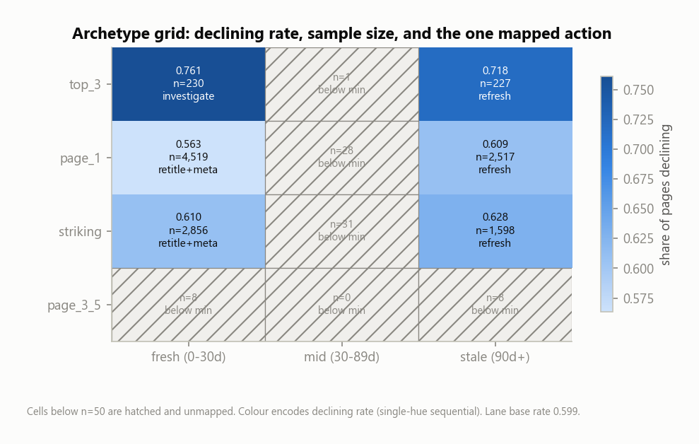
4. Route by archetype, not by score alone (observed, directional)
Position tier crossed with freshness band splits the queue into six archetypes with genuinely different decline rates, and each implies different work. Same score, different job.
| Archetype | n | decline rate | median CTR | median position | Action |
|---|---|---|---|---|---|
| top-3 / fresh (0–30d) | 230 | 0.761 | 0.20 | 2.4 | investigate |
| top-3 / stale (90d+) | 227 | 0.718 | 0.20 | 2.4 | refresh |
| striking distance / stale (90d+) | 1,598 | 0.628 | 0.18 | 14.8 | refresh |
| striking distance / fresh (0–30d) | 2,856 | 0.610 | 0.17 | 13.5 | retitle + meta |
| page-1 / stale (90d+) | 2,517 | 0.609 | 0.21 | 6.0 | refresh |
| page-1 / fresh (0–30d) | 4,519 | 0.563 | 0.26 | 6.7 | retitle + meta |
The most urgent archetype is the least intuitive one: pages already sitting in the top three, recently updated, and still slipping. Nothing about them looks like a problem, which is precisely why they need a human to look.
5. Trust four reason codes; treat two as context only (observed, directional)
Of the eight reason codes attached to queued items, six sit above base rate — but only
four by a margin worth acting on. stale_90plus (+0.023) and
striking_distance (+0.019) clear it by less than a third of what the weakest of the
four manages, which is inside the noise these buckets carry; treat them as weak signals rather
than evidence. The remaining two sit measurably below base rate, and reading those as
evidence of risk would be a straightforward mistake.
| Reason code | n | decline rate | vs base rate | How to read it |
|---|---|---|---|---|
zero_clicks | 1,216 | 0.773 | +0.175 | risk signal |
thin_for_tier | 825 | 0.760 | +0.161 | risk signal |
zero_engagement | 6,324 | 0.660 | +0.062 | risk signal |
ctr_gap_vs_peers | 6,132 | 0.654 | +0.056 | risk signal |
stale_90plus | 4,350 | 0.621 | +0.023 | weak signal |
striking_distance | 3,840 | 0.618 | +0.019 | weak signal |
decay_zone_age | 6,771 | 0.553 | −0.046 | context only — not evidence of decline |
high_volume_leverage | 6,306 | 0.537 | −0.061 | context only — not evidence of decline |
A ninth code, stale_181plus, was dropped for failing the n ≥ 50
minimum. high_volume_leverage stays on the card because a reviewer needs it to judge
effort — a fix on a high-traffic page is worth more — but it describes payoff, not
risk, and it must not be read as the latter.
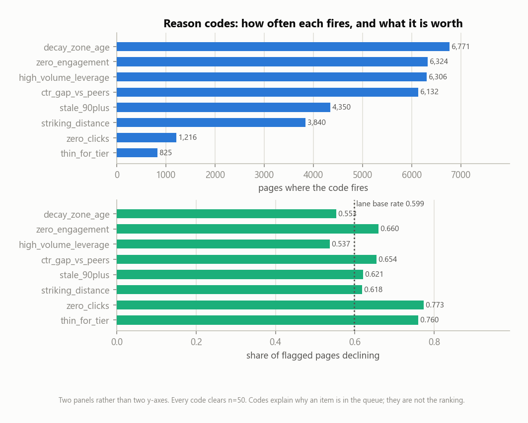
decay_zone_age is the most common code in the queue and sits
below the base rate; zero_clicks is among the rarest and carries the most
signal. Two panels rather than two y-axes, so neither scale distorts the other.6. Re-measure the base rate before trusting any precision number (measured)
The observed base rate ranges 0.485–0.747 across folds and 0.349–0.633 across fortnights. A precision@50 of 0.75 is excellent against a base rate of 0.49 and mediocre against 0.63. Report them together, or not at all.
7. Keep a human in front of every item (by design)
The reviewer's job is exactly the part the model cannot do: open the live snippet and judge whether the title genuinely mismatches the query intent; decide whether a page is dated or simply old; decide whether a competitor gap is realistically closable or whether position 11 is the ceiling for that query. Competitive difficulty is not in the feature set. Intent is not in the feature set. The queue orders the questions; the editor answers them.
When to stop trusting the queue
Every threshold below is a measured number, not a round one. A trigger set at "if performance drops a lot" fires never or always.
| Trigger | Threshold | Where the number comes from | Response |
|---|---|---|---|
| precision@50 below the grouped-fold floor | < 0.740 | five-fold grouped minimum | investigate before publishing the next queue |
| precision@50 reaches the rule's level | ≤ 0.672 | grouped mean of the Week-4 rule | revert to the rule — cheaper and explainable |
| precision@50 reaches the base rate | ≤ 0.599 | definitional | retire the queue; it adds nothing over any ordering |
| label base rate leaves its observed range | outside 0.485–0.747 | observed fold base rates | the population changed, not the model — retrain |
| feature drift | PSI > 0.20 | standard PSI bands | investigate; > 0.25 retrain |
| new clients look unlike training clients | adversarial AUC > 0.70 | adversarial validation | expect the measured new-client cost of 0.054 ROC AUC |
Back to the content problem
The question this started from was whether a learned ranking can beat a hand-written threshold rule at deciding which decaying page a human should fix first. On this data, the measured answer is yes, but by less than it first appears, and for a different reason than expected.
The gain over the rule is real and survives client-clustered resampling — a content operation reviewing fifty pages a cycle would find roughly 45 genuinely declining pages instead of 34. Across a year of weekly cycles that is a material difference in where editorial time lands. But the gain over a one-line heuristic is not measurable at that budget, and the gain from a bigger feature set is not measurable at all. The honest recommendation to a team in FlyRank's position is therefore narrower than "ship a model": replace the threshold rule with the smallest learned ranking you can defend, keep the rule live as the revert target, and spend the saved effort on the label rather than on the estimator.
That last point is where the study actually landed. The largest number in this entire investigation is not a model gap — it is the label's own base rate moving 0.349 to 0.633 between two consecutive fortnights, and a date-anchored feature drifting at PSI 8.49. For content decay specifically, when you measure moves the answer more than what you fit to it. A team investing here would get more from defining decay on a stable future window, and from running one controlled test of whether refreshing a queued page changes its trajectory, than from any further modelling. No such test exists in this work, which is why nothing in this paper claims a refresh causes recovery — only that these pages are the ones worth opening first.
8Reproducibility
Everything on this page traces to a committed file. Random seed 42 throughout;
scikit-learn 1.6.1; dependencies in
requirements.txt
with no additions beyond the starter set. From a fresh clone:
git clone https://github.com/mdsvr/flyrank && pip install -r requirements.txt,
then run the notebooks in order. The capstone notebook re-renders every table on this page from
the committed metrics files in seconds, without refitting anything — so the page and the
notebook cannot silently disagree.
| Notebook | What it establishes | Receipt it produced |
|---|---|---|
| w01_research_question | The question, the lane, and the three numbers that justified seven weeks on it | — |
| w02_ml_task_framing | Ranking, not classification; precision@50 named before any model existed | — |
| w03_data_contract | Grain, windows, field buckets, exclusions, three verification queries | — |
| w03_feature_leakage_check | Past→future feature vector; two deliberate leaks planted, detected and removed | — |
| w04_signal_audit | Three signal tests on the lane slice, one linked to a live product flag | — |
| w04_baseline_score | The transparent rule, its two signal checks, and a sceptical top-10 review | — |
| w05_model | First trained models on a hand-packed client-grouped split (three of its claims were later corrected; the corrections are recorded in the notebook header rather than edited away) | — |
| w06_validation_audit | Random vs client-grouped folds, the leakage re-hunt, adversarial validation | w06_split_comparison.json |
| w07_action_playbook | 16-config search, cluster bootstrap, time-aware 2×2, the queue and its figures | w07_model_search, w07_cluster_bootstrap, w07_time_aware, w07_playbook_metrics, w07_drift_baseline |
| capstone | Renders every table and figure on this page from the receipts above | the six figures in docs/img/ |
What is deliberately not in the repository. The ranked queue CSV. It carries pseudonymous client and content identifiers, and continuous integration fails if any dataset CSV is committed. It regenerates from the playbook notebook, which is the point: it is reproducible output, not an artifact to pass around. The metrics JSONs are the opposite — committed on purpose, so any number on this page can be checked without re-running anything.
9Acknowledgments & data credit
Built on the FlyRank ML Internship dataset — https://flyrank.ai — a pseudonymised release of roughly 79 million rows of production search and engagement data. Working on real production data, rather than a tidied teaching set, is what made most of the findings in this paper possible: the client imbalance, the measurement gaps, the drifting base rate and the near-perfect client separability are all properties of real inventory that a clean benchmark would have hidden.
Thanks to the FlyRank ML Internship programme for the dataset, the weekly structure, and the research paper whose exploratory appendix gave me two methodology questions to ask — and then made me ask the same two questions of my own model, which is where the retractions in §6 came from.